Consider a Hamiltonian  leading to the classical equations of motion
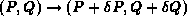
A class of second order algorithms for solving this equations of motion in discrete time steps is then given by
where the Hamiltonian 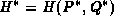 and its partial derivatives are taken
at the time-interpolated phase space point
and its partial derivatives are taken
at the time-interpolated phase space point
In order to resume the right differential equations in the continous
time limit 

is required. We note that if B=b=0, the recursion formula ( 2 ) is actually of first order.
The conserved Noether charge is the coefficient of the generators
of an infinitesimal transformation of the variables
 , which leaves the action,

invariant. Considering time independent transformations only, like those gauge transformations generated by the Gauss' law, it is equivalent to require that the Lagrangian is invariant,

For the class of algorithms under discussion one uses

deriving the discrete time step Noether charge. We get

which, upon using the equations of motion
( 2 ) for the substitution
of partial derivatives of the interpolated Hamiltonian  , reduces to
Our task is now to write it as a difference between copies of the same quantity at some later and earlier time around t

with  or 1,
where the
or 1,
where the  -s are the parameters of the infinitesimal
symmetry transformation --- like gauge transformation or norm conserving
unitary rotation --- and a summation over the index
-s are the parameters of the infinitesimal
symmetry transformation --- like gauge transformation or norm conserving
unitary rotation --- and a summation over the index  is understood.
The
is understood.
The  -s are then the correct expressions for the Noether charge
which is conserved by the discrete time step recursion formula.
-s are then the correct expressions for the Noether charge
which is conserved by the discrete time step recursion formula.
Using the class of algorithms we are discussing, we substitute  and
and
 from
eq.( 3 )
into the above expression of
from
eq.( 3 )
into the above expression of
 ( 9 ). We get
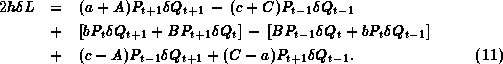
One easily realizes that in order to write the above expression in a form
of a difference between updated  and not yet updated
  terms the third line has to vanish. This requires c=A and a=C.
The second line is a difference between
terms the third line has to vanish. This requires c=A and a=C.
The second line is a difference between  and
and
 --- where
  ---
if b=B. From this contribution it follows a rate of change of the
Noether charge which has to vanish:
---
if b=B. From this contribution it follows a rate of change of the
Noether charge which has to vanish:

It requires the following definition:

Finally this definition coincides in the continous time limit
 with the correct Noether charge if b=1.
This identifies the first class of Noether charge conserving second
order time update algorithms:
with the correct Noether charge if b=1.
This identifies the first class of Noether charge conserving second
order time update algorithms:
Type I a=0 b=1 c=0 A=0 B=1 C=0.
Such algorithms are explicit and use even and odd time values for the update alternating.
The first line of the expression ( 11 )
also gives a proper difference
since due to A=c and C=a it is a+A=c+C.
These terms differ in their time argument with an amount of
2h --- meaning  --- relating t+1 and t-1 indices.
The definition
--- relating t+1 and t-1 indices.
The definition

leads to the first line of eq.( 11 ) considering its change from time t-1 to t+1,

and already coincides with the continous time definition. This defines the second class of Noether charge conserving update algorithms:
Type II a=C b=0 c=A A=c B=0 C=a.
Requiring the proper continuum limit for the equation of motion and the Noether charge also a+c=1 has to be fulfilled. Such algorithms are of first order only but always implicit.
Some of the generally known algorithms already satisfy the above conditions and belong to one of the above Type I or II classes. Type I is always an explicit algorithm --- using alternatively odd and even time points for the update procedure. In the present paper I refer this as the explizit odd even time algorithm, OET.
In the Type II class there is still a degree of freedom left in
specifying the update formulae (2,3).
The symmetric choice 
 which uses the arithmetic mean
of the already updated and not yet updated values in order to compute
their differences, is called here the implicit midpoint algorithm, IMP.
This is --- as its name suggests --- an inherently implicit algorithm,
which is too complicated for most systems showing nonlinear dynamics
and neighbour interconnections, especially for lattice gauge theory.
It is possible in some cases, like the harmonic oscillator, to convert
such algorithms in an explicit form analytically, but in most cases not.
which uses the arithmetic mean
of the already updated and not yet updated values in order to compute
their differences, is called here the implicit midpoint algorithm, IMP.
This is --- as its name suggests --- an inherently implicit algorithm,
which is too complicated for most systems showing nonlinear dynamics
and neighbour interconnections, especially for lattice gauge theory.
It is possible in some cases, like the harmonic oscillator, to convert
such algorithms in an explicit form analytically, but in most cases not.
It is also imaginable to use partially implicit versions of Type II algorithms. Since it is often the case --- like in lattice gauge theory --- that the Hamiltonian is a separable quadratic function of the canonical momenta P, but is a very complicated one with respect to the generalized coordinate Q, an algorithm explicit in Q but implicit in P or vice versa may be useful. This choice, belonging to a=1, c=0, is refered in the present paper as the half implicit half explicit endpoint algorithm, HIHEP.
Finally a general, mixed Type I and Type II algorithm also can be used with the general Noether charge definition
Its rate of change, 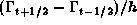 consists of the first two lines of eq.( 11 )
and it has the correct continuum limit if
a+b+c=1. We refer such general algorithms as Type III in the present
paper.
consists of the first two lines of eq.( 11 )
and it has the correct continuum limit if
a+b+c=1. We refer such general algorithms as Type III in the present
paper.
These algorithms, although in principle all of them conserves a discrete time Noether charge with the correct continuum limit, may be different in their performance with respect to stability and computational complexity. In the next Chapter we compare them in a test of describing simple dynamical systems.